
线性模型
用正规方程进行线性回归
import numpy as np
%matplotlib inline
import matplotlib
import matplotlib.pyplot as plt

X = 2*np.random.rand(100, 1)  #单纯的生成2*(0——1)的随机数,规模为100*1
y = 4 + 3 * X + np.random.randn(100, 1) #randn服从标准正态分布
plt.plot(X, y, "b.")
plt.xlabel("$x_1$", fontsize=18)
plt.ylabel("$y$", rotation=0, fontsize=18)
plt.axis([0, 2, 0, 15])
plt.show()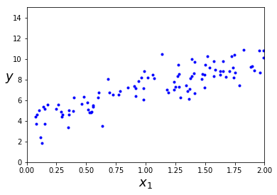
X_b = np.c_[np.ones((100,1)), X] #添加一列全1列在X左边,不添的话回归方程则没有偏置项
theta_best = np.linalg.inv(X_b.T.dot(X_b)).dot(X_b.T).dot(y)
theta_best
array([[ 4.0224133],
[ 3.0375984]])X_new = np.array([[0],[2]])
X_new_b = np.c_[np.ones((2,1)),X_new] #这才是实例的向量形式
y_predict = X_new_b.dot(theta_best)
y_predictarray([[ 4.0224133 ],
[ 10.09761009]])plt.plot(X, y, "b.")
plt.xlabel("$x_1$", fontsize=18)
plt.ylabel("$y$", rotation=0, fontsize=18)
plt.axis([0, 2, 0, 15])
plt.plot(X_new, y_predict,"r-")
plt.show()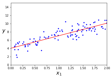
用模型进行线性回归
from sklearn.linear_model import LinearRegression

lin_reg = LinearRegression()
lin_reg.fit(X,y)
lin_reg.intercept_,lin_reg.coef_  #intercept截距,coef系数
(array([ 4.0224133]), array([[ 3.0375984]]))lin_reg.predict(X_new) #预测得和正规方程一样,不过这是基于SVD矩阵分解的array([[ 4.0224133 ],
[ 10.09761009]])用批量梯度下降进行线性回归
eta = 0.1 #study rate
n_iterations = 10000
m = 100 #the number of train example
theta = np.random.randn(2,1) #随机初始值

for iteration in range(n_iterations):
    gradients = 2/m * X_b.T.dot(X_b.dot(theta) -y)  #均方误差的偏导数
    theta = theta - eta * gradients
theta #最后得到theta的优化值array([[ 4.0224133],
[ 3.0375984]])探索批量梯度下降
过程
- 随机选取一个 theta
- 用整个训练集求出一个固定的梯度
- 递归优化 theta
theta_path_bgd = []   #存储theta的过程值
def plot_gradient_descent(theta, eta, theta_path = None):
    m = len(X_b)
    plt.plot(X, y, "b.")
    n_iterations = 1000
    for iteration in range(n_iterations):
        if iteration < 10:
            y_predict = X_new_b.dot(theta)
            style = "b-" if iteration > 0 else "r--"
            plt.plot(X_new, y_predict, style)
        gradients = 2/m * X_b.T.dot(X_b.dot(theta) - y)
        theta = theta - eta * gradients
        if theta_path is not None:
            theta_path.append(theta)
    plt.xlabel("$X_1$", fontsize = 18)
    plt.axis([0,2,0,15])
plt.title(r"$\eta$ = {}".format(eta), fontsize = 16)np.random.seed(42)
theta = np.random.randn(2,1)
plt.figure(figsize=(10,4))
plt.subplot(131); plot_gradient_descent(theta, eta=0.02)
plt.ylabel("$y$", rotation=0, fontsize=18)
plt.subplot(132); plot_gradient_descent(theta, eta=0.1, theta_path=theta_path_bgd)
plt.subplot(133); plot_gradient_descent(theta, eta=0.5)
plt.show()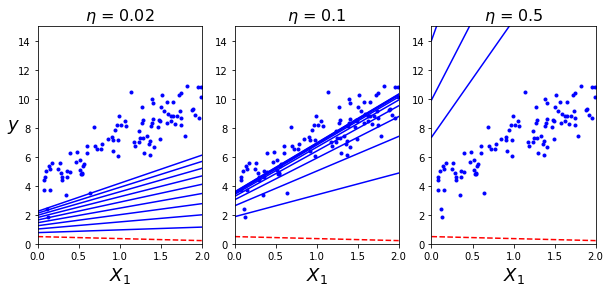
[array([[ 1.86730689],
	   [ 1.50575404]]), array([[ 2.61930247],
	   [ 2.39396727]]), array([[ 3.03478759],
	  .......
表明学习率
随机梯度下降
过程
- 随机选个 theta
- 在训练集中随机选一个点求出其梯度
- 随着迭代次数增加降低学习率
- 递归优化 theta
theta_path_sgd = []
m = len(X_b)
np.random.seed(42)
n_epochs = 50
t0, t1 = 5, 50  # learning schedule hyperparameters

def learning_schedule(t):
    return t0 / (t + t1)

theta = np.random.randn(2,1)  # random initialization

for epoch in range(n_epochs):
    for i in range(m):
        if epoch <50 and i < 20:
            y_predict = X_new_b.dot(theta)
            style = "b-" if i > 0 else "r--"
            plt.plot(X_new, y_predict, style)
    random_index = np.random.randint(m)
    xi = X_b[random_index:random_index+1]
    yi = y[random_index:random_index+1]
    gradients = 2 * xi.T.dot(xi.dot(theta) - yi)    #梯度是随机选一个点进行计算
    eta = learning_schedule(epoch + i)           #学习率随着迭代次数增加而增加
    theta = theta - eta * gradients
    theta_path_sgd.append(theta)

plt.plot(X, y, "b.")
plt.xlabel("$x_1$", fontsize=18)
plt.ylabel("$y$", rotation=0, fontsize=18)
plt.axis([0, 2, 0, 15])
plt.show()           #学习率过早减小导致下图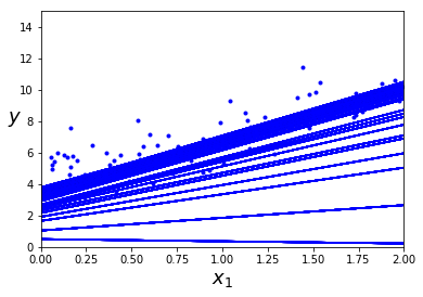
thetaarray([[ 3.84494505],
[ 3.27773445]])from sklearn.linear_model import SGDRegressor
sgd_reg = SGDRegressor(max_iter=50, penalty=None, eta0=0.1, random_state=42)
sgd_reg.fit(X, y.ravel())SGDRegressor(alpha=0.0001, average=False, early_stopping=False, epsilon=0.1,
eta0=0.1, fit_intercept=True, l1_ratio=0.15,
learning_rate='invscaling', loss='squared_loss', max_iter=50,
n_iter=None, n_iter_no_change=5, penalty=None, power_t=0.25,
random_state=42, shuffle=True, tol=None, validation_fraction=0.1,
verbose=0, warm_start=False)sgd_reg.intercept_,sgd_reg.coef_ # (array([ 4.15885372]), array([ 2.78382451]))y.ravel()array([ 7.92135333, 8.56691098, 5.99502404, 5.41513681,
6.44148562, 4.86811936, 7.10136485, 3.42339943,
3.67839599, 3.33761007, 10.60499941, 9.85896324,
5.24987976, 6.41309292, 8.27404813, 10.2284994 ,
7.36249471, 5.53075467, 5.82242636, 8.73811634,
7.71831938, 5.68942818, 5.53702494, 9.31348781,
6.38312742, 4.65636541, 6.822189 , 7.57527945,
5.09018294, 8.20892064, 5.26167648, 9.31611915,
8.25069641, 6.20716153, 4.74007077, 4.21154293,
5.47356181, 3.65836925, 4.49619836, 10.47303379,
4.04746793, 7.79850061, 5.65985419, 4.04421099,
4.87118555, 9.47709443, 4.84031852, 3.17888951,
8.07583515, 7.40261652, 5.9161954 , 8.05550747,
6.00742713, 7.663237 , 7.18763962, 6.41589604,
3.6484945 , 7.5615348 , 6.90866543, 4.66088275,
11.41090766, 8.55184292, 4.54870059, 5.88453553,
6.50245164, 8.94983926, 8.9836167 , 7.81270696,
4.19772038, 3.87984973, 5.78906629, 8.39476674,
5.68339181, 8.74063201, 8.90028377, 5.26353559,
5.56526364, 6.71891745, 9.75285961, 5.96614923,
4.63267988, 8.25034491, 8.51859076, 4.67946486,
8.49665663, 5.23937975, 4.98571677, 8.24719202,
9.71403888, 8.88804298, 4.58339356, 9.07247433,
6.27455895, 9.07438272, 10.39908052, 5.87060124,
8.06497982, 4.13650819, 8.94576743, 8.60587748])小批量梯度下降
theta_path_mgd = []

n_iterations = 50
minibatch_size = 20

np.random.seed(42)
theta = np.random.randn(2,1)  # random initialization

t0, t1 = 200, 1000
def learning_schedule(t):
    return t0 / (t + t1)

t = 0
for epoch in range(n_iterations):
    shuffled_indices = np.random.permutation(m)
    X_b_shuffled = X_b[shuffled_indices]
    y_shuffled = y[shuffled_indices]
    for i in range(0, m, minibatch_size):
        t += 1
        xi = X_b_shuffled[i:i+minibatch_size]
        yi = y_shuffled[i:i+minibatch_size]
        gradients = 2/minibatch_size * xi.T.dot(xi.dot(theta) - yi)
        eta = learning_schedule(t)
        theta = theta - eta * gradients
theta_path_mgd.append(theta)thetaarray([[ 4.21526857],
[ 2.81576239]])theta_path_bgd = np.array(theta_path_bgd)
theta_path_sgd = np.array(theta_path_sgd)
theta_path_mgd = np.array(theta_path_mgd)
plt.figure(figsize=(7,4))
plt.plot(theta_path_sgd[:, 0], theta_path_sgd[:, 1], "r-s", linewidth=1, label="Stochastic")
plt.plot(theta_path_mgd[:, 0], theta_path_mgd[:, 1], "g-+", linewidth=2, label="Mini-batch")
plt.plot(theta_path_bgd[:, 0], theta_path_bgd[:, 1], "b-o", linewidth=3, label="Batch")
plt.legend(loc="upper left", fontsize=16)
plt.xlabel(r"$\theta_0$", fontsize=20)
plt.ylabel(r"$\theta_1$ ", fontsize=20, rotation=0)
plt.axis([2.5, 4.5, 2.3, 3.9])
plt.show()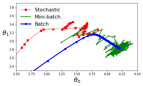
多项式回归
import numpy as np
import numpy.random as rnd
np.random.seed(42)

m = 100
X = 6 * np.random.rand(m, 1) - 3
y = 0.5 * X**2 + X + 2 + np.random.randn(m, 1)

plt.plot(X, y, "b.")
plt.xlabel("$x_1$", fontsize=18)
plt.ylabel("$y$", rotation=0, fontsize=18)
plt.axis([-3, 3, 0, 10])
plt.show()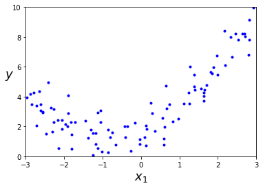
from sklearn.preprocessing import PolynomialFeatures
poly_features = PolynomialFeatures(degree=2, include_bias=False)
X_poly = poly_features.fit_transform(X)
X[0] # array([-0.75275929])X_poly[0] # array([-0.75275929, 0.56664654])lin_reg = LinearRegression()
lin_reg.fit(X_poly, y)
lin_reg.intercept_, lin_reg.coef_ # (array([ 1.78134581]), array([[ 0.93366893, 0.56456263]]))X_new=np.linspace(-3, 3, 100).reshape(100, 1)
X_new_poly = poly_features.transform(X_new)
y_new = lin_reg.predict(X_new_poly)
plt.plot(X, y, "b.")
plt.plot(X_new, y_new, "r-", linewidth=2, label="Predictions")
plt.xlabel("$x_1$", fontsize=18)
plt.ylabel("$y$", rotation=0, fontsize=18)
plt.legend(loc="upper left", fontsize=14)
plt.axis([-3, 3, 0, 10])
plt.show()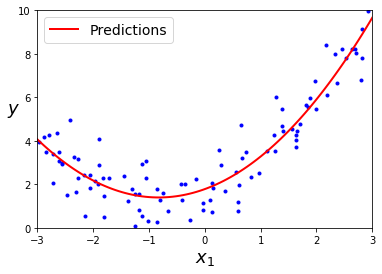
from sklearn.preprocessing import StandardScaler
from sklearn.pipeline import Pipeline

for style, width, degree in (("g-", 1, 300), ("b--", 2, 2), ("r-+", 2, 1)):
    polybig_features = PolynomialFeatures(degree=degree, include_bias=False)
    std_scaler = StandardScaler()
    lin_reg = LinearRegression()
    polynomial_regression = Pipeline([
            ("poly_features", polybig_features),
            ("std_scaler", std_scaler),
            ("lin_reg", lin_reg),
        ])
    polynomial_regression.fit(X, y)
    y_newbig = polynomial_regression.predict(X_new)
    plt.plot(X_new, y_newbig, style, label=str(degree), linewidth=width)

plt.plot(X, y, "b.", linewidth=3)
plt.legend(loc="upper left")
plt.xlabel("$x_1$", fontsize=18)
plt.ylabel("$y$", rotation=0, fontsize=18)
plt.axis([-3, 3, 0, 10])
plt.show()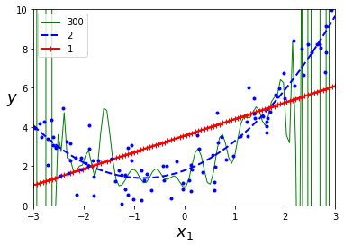
from sklearn.metrics import mean_squared_error
from sklearn.model_selection import train_test_split

def plot_learning_curves(model, X, y):
    X_train, X_val, y_train, y_val = train_test_split(X, y, test_size=0.2, random_state=10)
    train_errors, val_errors = [], []
    for m in range(1, len(X_train)):
        model.fit(X_train[:m], y_train[:m])
        y_train_predict = model.predict(X_train[:m])
        y_val_predict = model.predict(X_val)
        train_errors.append(mean_squared_error(y_train[:m], y_train_predict))
        val_errors.append(mean_squared_error(y_val, y_val_predict))

    plt.plot(np.sqrt(train_errors), "r-+", linewidth=2, label="train")
    plt.plot(np.sqrt(val_errors), "b-", linewidth=3, label="val")
    plt.legend(loc="upper right", fontsize=14)   # not shown in the book
    plt.xlabel("Training set size", fontsize=14) # not shown
    plt.ylabel("RMSE", fontsize=14)              # not shown
lin_reg = LinearRegression()
plot_learning_curves(lin_reg, X, y)
plt.axis([0, 80, 0, 3]) # not shown in the book
plt.show() # not shown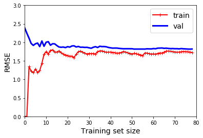
from sklearn.pipeline import Pipeline

polynomial_regression = Pipeline([
        ("poly_features", PolynomialFeatures(degree=10, include_bias=False)),
        ("lin_reg", LinearRegression()),
    ])

plot_learning_curves(polynomial_regression, X, y)
plt.axis([0, 80, 0, 3])           # not shown
plt.show()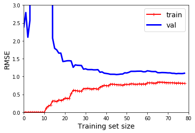
正则化模型
from sklearn.linear_model import Ridge

np.random.seed(42)
m = 20
X = 3 * np.random.rand(m, 1)
y = 1 + 0.5 * X + np.random.randn(m, 1) / 1.5
X_new = np.linspace(0, 3, 100).reshape(100, 1)

def plot_model(model_class, polynomial, alphas, **model_kargs):
    for alpha, style in zip(alphas, ("b-", "g--", "r:")):
        model = model_class(alpha, **model_kargs) if alpha > 0 else LinearRegression()
        if polynomial:
            model = Pipeline([
                    ("poly_features", PolynomialFeatures(degree=10, include_bias=False)),
                    ("std_scaler", StandardScaler()),
                    ("regul_reg", model),
                ])
        model.fit(X, y)
        y_new_regul = model.predict(X_new)
        lw = 2 if alpha > 0 else 1
        plt.plot(X_new, y_new_regul, style, linewidth=lw, label=r"$\alpha = {}$".format(alpha))
    plt.plot(X, y, "b.", linewidth=3)
    plt.legend(loc="upper left", fontsize=15)
    plt.xlabel("$x_1$", fontsize=18)
    plt.axis([0, 3, 0, 4])

plt.figure(figsize=(8,4))
plt.subplot(121)
plot_model(Ridge, polynomial=False, alphas=(0, 10, 100), random_state=42)
plt.ylabel("$y$", rotation=0, fontsize=18)
plt.subplot(122)
plot_model(Ridge, polynomial=True, alphas=(0, 10**-5, 1), random_state=42)
plt.show()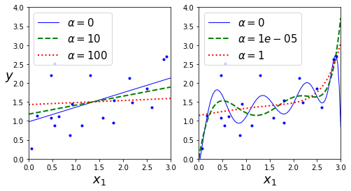
from sklearn.linear_model import Ridge
ridge_reg = Ridge(alpha=1, solver="cholesky", random_state=42)
ridge_reg.fit(X, y)
ridge_reg.predict([[1.5]]) #    array([[ 1.55071465]])
sgd_reg = SGDRegressor(max_iter=5, penalty="l2", random_state=42)
sgd_reg.fit(X, y.ravel())
sgd_reg.predict([[1.5]]) # array([ 1.13500145])ridge_reg = Ridge(alpha=1, solver="sag", random_state=42)
ridge_reg.fit(X, y)
ridge_reg.predict([[1.5]]) # array([[ 1.5507201]])from sklearn.linear_model import Lasso
plt.figure(figsize=(8,4))
plt.subplot(121)
plot_model(Lasso, polynomial=False, alphas=(0, 0.1, 1), random_state=42)
plt.ylabel("$y$", rotation=0, fontsize=18)
plt.subplot(122)
plot_model(Lasso, polynomial=True, alphas=(0, 10**-7, 1), tol=1, random_state=42)
plt.show()
from sklearn.linear_model import Lasso
lasso_reg = Lasso(alpha=0.1)
lasso_reg.fit(X, y)
lasso_reg.predict([[1.5]]) #    array([ 1.53788174])
from sklearn.linear_model import ElasticNet
elastic_net = ElasticNet(alpha=0.1, l1_ratio=0.5, random_state=42)
elastic_net.fit(X, y)
elastic_net.predict([[1.5]]) # array([ 1.54333232])np.random.seed(42)
m = 100
X = 6 * np.random.rand(m, 1) - 3
y = 2 + X + 0.5 * X**2 + np.random.randn(m, 1)
X_train, X_val, y_train, y_val = train_test_split(X[:50], y[:50].ravel(), test_size=0.5, random_state=10)
poly_scaler = Pipeline([
("poly_features", PolynomialFeatures(degree=90, include_bias=False)),
("std_scaler", StandardScaler()),
])
X_train_poly_scaled = poly_scaler.fit_transform(X_train)
X_val_poly_scaled = poly_scaler.transform(X_val)
sgd_reg = SGDRegressor(max_iter=1,
penalty=None,
eta0=0.0005,
warm_start=True,
learning_rate="constant",
random_state=42)
n_epochs = 500
train_errors, val_errors = [], []
for epoch in range(n_epochs):
sgd_reg.fit(X_train_poly_scaled, y_train)
y_train_predict = sgd_reg.predict(X_train_poly_scaled)
y_val_predict = sgd_reg.predict(X_val_poly_scaled)
train_errors.append(mean_squared_error(y_train, y_train_predict))
val_errors.append(mean_squared_error(y_val, y_val_predict))
best_epoch = np.argmin(val_errors)
best_val_rmse = np.sqrt(val_errors[best_epoch])
plt.annotate('Best model',
xy=(best_epoch, best_val_rmse),
xytext=(best_epoch, best_val_rmse + 1),
ha="center",
arrowprops=dict(facecolor='black', shrink=0.05),
fontsize=16,
)
best_val_rmse -= 0.03 # just to make the graph look better
plt.plot([0, n_epochs], [best_val_rmse, best_val_rmse], "k:", linewidth=2)
plt.plot(np.sqrt(val_errors), "b-", linewidth=3, label="Validation set")
plt.plot(np.sqrt(train_errors), "r--", linewidth=2, label="Training set")
plt.legend(loc="upper right", fontsize=14)
plt.xlabel("Epoch", fontsize=14)
plt.ylabel("RMSE", fontsize=14)
plt.show()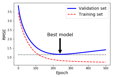
from sklearn.base import clone
sgd_reg = SGDRegressor(max_iter=1, warm_start=True, penalty=None,
                       learning_rate="constant", eta0=0.0005, random_state=42)

minimum_val_error = float("inf")
best_epoch = None
best_model = None
for epoch in range(1000):
    sgd_reg.fit(X_train_poly_scaled, y_train)  # continues where it left off
    y_val_predict = sgd_reg.predict(X_val_poly_scaled)
    val_error = mean_squared_error(y_val, y_val_predict)
    if val_error < minimum_val_error:
        minimum_val_error = val_error
        best_epoch = epoch
        best_model = clone(sgd_reg)
best_epoch, best_model(239,
SGDRegressor(alpha=0.0001, average=False, early_stopping=False, epsilon=0.1,
eta0=0.0005, fit_intercept=True, l1_ratio=0.15,
learning_rate='constant', loss='squared_loss', max_iter=1,
n_iter=None, n_iter_no_change=5, penalty=None, power_t=0.25,
random_state=42, shuffle=True, tol=None, validation_fraction=0.1,
verbose=0, warm_start=True))%matplotlib inline
import matplotlib.pyplot as plt
import numpy as npt1a, t1b, t2a, t2b = -1, 3, -1.5, 1.5
# ignoring bias term
t1s = np.linspace(t1a, t1b, 500)
t2s = np.linspace(t2a, t2b, 500)
t1, t2 = np.meshgrid(t1s, t2s)
T = np.c_[t1.ravel(), t2.ravel()]
Xr = np.array([[-1, 1], [-0.3, -1], [1, 0.1]])
yr = 2 * Xr[:, :1] + 0.5 * Xr[:, 1:]
J = (1/len(Xr) * np.sum((T.dot(Xr.T) - yr.T)**2, axis=1)).reshape(t1.shape)
N1 = np.linalg.norm(T, ord=1, axis=1).reshape(t1.shape)
N2 = np.linalg.norm(T, ord=2, axis=1).reshape(t1.shape)
t_min_idx = np.unravel_index(np.argmin(J), J.shape)
t1_min, t2_min = t1[t_min_idx], t2[t_min_idx]
t_init = np.array([[0.25], [-1]])def bgd_path(theta, X, y, l1, l2, core = 1, eta = 0.1, n_iterations = 50):
path = [theta]
for iteration in range(n_iterations):
gradients = core * 2/len(X) * X.T.dot(X.dot(theta) - y) + l1 * np.sign(theta) + 2 * l2 * theta
theta = theta - eta * gradients
path.append(theta)
return np.array(path)
plt.figure(figsize=(12, 8))
for i, N, l1, l2, title in ((0, N1, 0.5, 0, "Lasso"), (1, N2, 0, 0.1, "Ridge")):
JR = J + l1 * N1 + l2 * N2**2
tr_min_idx = np.unravel_index(np.argmin(JR), JR.shape)
t1r_min, t2r_min = t1[tr_min_idx], t2[tr_min_idx]
levelsJ=(np.exp(np.linspace(0, 1, 20)) - 1) * (np.max(J) - np.min(J)) + np.min(J)
levelsJR=(np.exp(np.linspace(0, 1, 20)) - 1) * (np.max(JR) - np.min(JR)) + np.min(JR)
levelsN=np.linspace(0, np.max(N), 10)
path_J = bgd_path(t_init, Xr, yr, l1=0, l2=0)
path_JR = bgd_path(t_init, Xr, yr, l1, l2)
path_N = bgd_path(t_init, Xr, yr, np.sign(l1)/3, np.sign(l2), core=0)
plt.subplot(221 + i * 2)
plt.grid(True)
plt.axhline(y=0, color='k')
plt.axvline(x=0, color='k')
plt.contourf(t1, t2, J, levels=levelsJ, alpha=0.9)
plt.contour(t1, t2, N, levels=levelsN)
plt.plot(path_J[:, 0], path_J[:, 1], "w-o")
plt.plot(path_N[:, 0], path_N[:, 1], "y-^")
plt.plot(t1_min, t2_min, "rs")
plt.title(r"$\ell_{}$ penalty".format(i + 1), fontsize=16)
plt.axis([t1a, t1b, t2a, t2b])
if i == 1:
plt.xlabel(r"$\theta_1$", fontsize=20)
plt.ylabel(r"$\theta_2$", fontsize=20, rotation=0)
plt.subplot(222 + i * 2)
plt.grid(True)
plt.axhline(y=0, color='k')
plt.axvline(x=0, color='k')
plt.contourf(t1, t2, JR, levels=levelsJR, alpha=0.9)
plt.plot(path_JR[:, 0], path_JR[:, 1], "w-o")
plt.plot(t1r_min, t2r_min, "rs")
plt.title(title, fontsize=16)
plt.axis([t1a, t1b, t2a, t2b])
if i == 1:
plt.xlabel(r"$\theta_1$", fontsize=20)
plt.show()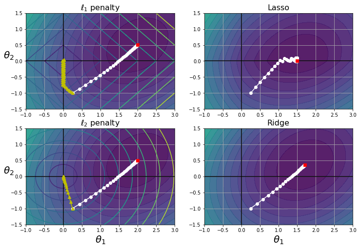
逻辑回归
t = np.linspace(-10, 10, 100)
sig = 1 / (1 + np.exp(-t))
plt.figure(figsize=(9, 3))
plt.plot([-10, 10], [0, 0], "k-")
plt.plot([-10, 10], [0.5, 0.5], "k:")
plt.plot([-10, 10], [1, 1], "k:")
plt.plot([0, 0], [-1.1, 1.1], "k-")
plt.plot(t, sig, "b-", linewidth=2, label=r"$\sigma(t) = \frac{1}{1 + e^{-t}}$")
plt.xlabel("t")
plt.legend(loc="upper left", fontsize=20)
plt.axis([-10, 10, -0.1, 1.1])
plt.show()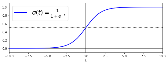
from sklearn import datasets
iris = datasets.load_iris()
list(iris.keys()) # ['data', 'target', 'target_names', 'DESCR', 'feature_names', 'filename']print(iris.DESCR).. _iris_dataset:
Iris plants dataset
--------------------
**Data Set Characteristics:**
:Number of Instances: 150 (50 in each of three classes)
:Number of Attributes: 4 numeric, predictive attributes and the class
:Attribute Information:
- sepal length in cm
- sepal width in cm
- petal length in cm
- petal width in cm
- class:
- Iris-Setosa
- Iris-Versicolour
- Iris-Virginica
:Summary Statistics:
============== ==== ==== ======= ===== ====================
Min Max Mean SD Class Correlation
============== ==== ==== ======= ===== ====================
sepal length: 4.3 7.9 5.84 0.83 0.7826
sepal width: 2.0 4.4 3.05 0.43 -0.4194
petal length: 1.0 6.9 3.76 1.76 0.9490 (high!)
petal width: 0.1 2.5 1.20 0.76 0.9565 (high!)
============== ==== ==== ======= ===== ====================
:Missing Attribute Values: None
:Class Distribution: 33.3% for each of 3 classes.
:Creator: R.A. Fisher
:Donor: Michael Marshall (MARSHALL%PLU@io.arc.nasa.gov)
:Date: July, 1988
The famous Iris database, first used by Sir R.A. Fisher. The dataset is taken
from Fisher's paper. Note that it's the same as in R, but not as in the UCI
Machine Learning Repository, which has two wrong data points.
This is perhaps the best known database to be found in the
pattern recognition literature. Fisher's paper is a classic in the field and
is referenced frequently to this day. (See Duda & Hart, for example.) The
data set contains 3 classes of 50 instances each, where each class refers to a
type of iris plant. One class is linearly separable from the other 2; the
latter are NOT linearly separable from each other.
.. topic:: References
- Fisher, R.A. "The use of multiple measurements in taxonomic problems"
Annual Eugenics, 7, Part II, 179-188 (1936); also in "Contributions to
Mathematical Statistics" (John Wiley, NY, 1950).
- Duda, R.O., & Hart, P.E. (1973) Pattern Classification and Scene Analysis.
(Q327.D83) John Wiley & Sons. ISBN 0-471-22361-1. See page 218.
- Dasarathy, B.V. (1980) "Nosing Around the Neighborhood: A New System
Structure and Classification Rule for Recognition in Partially Exposed
Environments". IEEE Transactions on Pattern Analysis and Machine
Intelligence, Vol. PAMI-2, No. 1, 67-71.
- Gates, G.W. (1972) "The Reduced Nearest Neighbor Rule". IEEE Transactions
on Information Theory, May 1972, 431-433.
- See also: 1988 MLC Proceedings, 54-64. Cheeseman et al"s AUTOCLASS II
conceptual clustering system finds 3 classes in the data.
- Many, many more ...X = iris["data"][:, 3:] # petal width
y = (iris["target"] == 2).astype(np.int) # 1 if Iris-Virginica, else 0from sklearn.linear_model import LogisticRegression
log_reg = LogisticRegression(random_state=42)
log_reg.fit(X, y)LogisticRegression(C=1.0, class_weight=None, dual=False, fit_intercept=True,
intercept_scaling=1, max_iter=100, multi_class='warn',
n_jobs=None, penalty='l2', random_state=42, solver='warn',
tol=0.0001, verbose=0, warm_start=False)X_new = np.linspace(0, 3, 1000).reshape(-1, 1)
y_proba = log_reg.predict_proba(X_new)
plt.plot(X_new, y_proba[:, 1], "g-", linewidth=2, label="Iris-Virginica")
plt.plot(X_new, y_proba[:, 0], "b--", linewidth=2, label="Not Iris-Virginica")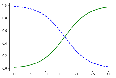
X_new = np.linspace(0, 3, 1000).reshape(-1, 1)
y_proba = log_reg.predict_proba(X_new)
decision_boundary = X_new[y_proba[:, 1] >= 0.5][0]

plt.figure(figsize=(8, 3))
plt.plot(X[y==0], y[y==0], "bs")
plt.plot(X[y==1], y[y==1], "g^")
plt.plot([decision_boundary, decision_boundary], [-1, 2], "k:", linewidth=2)
plt.plot(X_new, y_proba[:, 1], "g-", linewidth=2, label="Iris-Virginica")
plt.plot(X_new, y_proba[:, 0], "b--", linewidth=2, label="Not Iris-Virginica")
plt.text(decision_boundary+0.02, 0.15, "Decision  boundary", fontsize=14, color="k", ha="center")
plt.arrow(decision_boundary, 0.08, -0.3, 0, head_width=0.05, head_length=0.1, fc='b', ec='b')
plt.arrow(decision_boundary, 0.92, 0.3, 0, head_width=0.05, head_length=0.1, fc='g', ec='g')
plt.xlabel("Petal width (cm)", fontsize=14)
plt.ylabel("Probability", fontsize=14)
plt.legend(loc="center left", fontsize=14)
plt.axis([0, 3, -0.02, 1.02])
plt.show()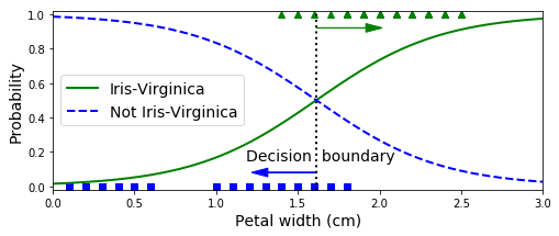
decision_boundary # array([ 1.61561562])log_reg.predict([[1.7], [1.5]]) # array([1, 0])from sklearn.linear_model import LogisticRegression
X = iris["data"][:, (2, 3)] # petal length, petal width
y = (iris["target"] == 2).astype(np.int)
log_reg = LogisticRegression(C=10**10, random_state=42)
log_reg.fit(X, y)
x0, x1 = np.meshgrid(
np.linspace(2.9, 7, 500).reshape(-1, 1),
np.linspace(0.8, 2.7, 200).reshape(-1, 1),
)
X_new = np.c_[x0.ravel(), x1.ravel()]
y_proba = log_reg.predict_proba(X_new)
plt.figure(figsize=(10, 4))
plt.plot(X[y==0, 0], X[y==0, 1], "bs")
plt.plot(X[y==1, 0], X[y==1, 1], "g^")
zz = y_proba[:, 1].reshape(x0.shape)
contour = plt.contour(x0, x1, zz, cmap=plt.cm.brg)
left_right = np.array([2.9, 7])
boundary = -(log_reg.coef_[0][0] * left_right + log_reg.intercept_[0]) / log_reg.coef_[0][1]
plt.clabel(contour, inline=1, fontsize=12)
plt.plot(left_right, boundary, "k--", linewidth=3)
plt.text(3.5, 1.5, "Not Iris-Virginica", fontsize=14, color="b", ha="center")
plt.text(6.5, 2.3, "Iris-Virginica", fontsize=14, color="g", ha="center")
plt.xlabel("Petal length", fontsize=14)
plt.ylabel("Petal width", fontsize=14)
plt.axis([2.9, 7, 0.8, 2.7])
plt.show()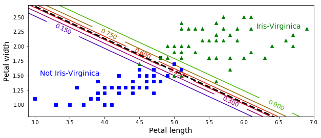
X = iris["data"][:, (2, 3)]  # petal length, petal width
y = iris["target"]

softmax_reg = LogisticRegression(multi_class="multinomial",solver="lbfgs", C=10, random_state=42)
softmax_reg.fit(X, y)
LogisticRegression(C=10, class_weight=None, dual=False, fit_intercept=True,
intercept_scaling=1, max_iter=100, multi_class='multinomial',
n_jobs=None, penalty='l2', random_state=42, solver='lbfgs',
tol=0.0001, verbose=0, warm_start=False)x0, x1 = np.meshgrid(
np.linspace(0, 8, 500).reshape(-1, 1),
np.linspace(0, 3.5, 200).reshape(-1, 1),
)
X_new = np.c_[x0.ravel(), x1.ravel()]
y_proba = softmax_reg.predict_proba(X_new)
y_predict = softmax_reg.predict(X_new)
zz1 = y_proba[:, 1].reshape(x0.shape)
zz = y_predict.reshape(x0.shape)
plt.figure(figsize=(10, 4))
plt.plot(X[y==2, 0], X[y==2, 1], "g^", label="Iris-Virginica")
plt.plot(X[y==1, 0], X[y==1, 1], "bs", label="Iris-Versicolor")
plt.plot(X[y==0, 0], X[y==0, 1], "yo", label="Iris-Setosa")
from matplotlib.colors import ListedColormap
custom_cmap = ListedColormap(['#fafab0','#9898ff','#a0faa0'])
plt.contourf(x0, x1, zz, cmap=custom_cmap)
contour = plt.contour(x0, x1, zz1, cmap=plt.cm.brg)
plt.clabel(contour, inline=1, fontsize=12)
plt.xlabel("Petal length", fontsize=14)
plt.ylabel("Petal width", fontsize=14)
plt.legend(loc="center left", fontsize=14)
plt.axis([0, 7, 0, 3.5])
plt.show()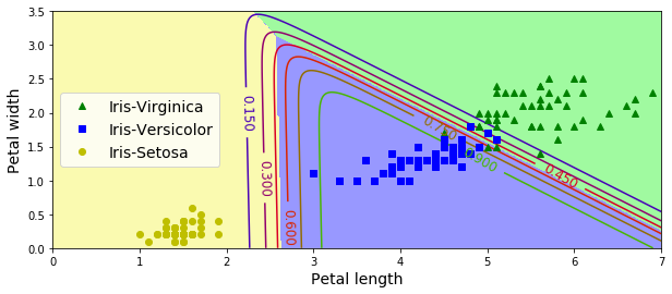
softmax_reg.predict([[5, 2]]) # array([2])softmax_reg.predict_proba([[5, 2]]) # array([[ 6.38014896e-07, 5.74929995e-02, 9.42506362e-01]])