机器学习基本流程

以泰坦尼克号乘客存活率为例

大纲：

宏观上定义问题，明确目标，选择性能指标，检查假设的合理性。
建立工作空间，加载数据集，浏览数据结构和含义，划分测试集。
探索性数据可视化，发现数据之间的关系，实验数据组合。
数据清洗，处理非数字类型数据，建立处理管道，为后续算法做准备。
选择和训练模型，计算性能指标，进行交叉验证，保存模型。
优化模型，网格搜索，随即搜索，集成方法等，并分析出最好的模型或模型组合，计算出性能指标。
加载，监控，维持系统的稳定性。

定义问题

问题描述： RMS 泰坦尼克号的沉没是历史上最臭名昭着的沉船之一。 1912 年 4 月 15 日，在她的处女航中，泰坦尼克号在与冰山相撞后沉没，在 2224 名船员造成 1502 人死亡。这场耸人听闻的悲剧震惊了国际社会，并为船舶制定了更好的安全规定。船舶残骸造成这种生命损失的原因之一是乘客和船员没有足够的救生艇。虽然有一些运气因素涉及到沉没，但有些人比其他人更容易生存，比如妇女，儿童和上流社会。在这次挑战中，我们要求您完成对哪些人可能存活的分析。特别是，我们要求您运用机器学习工具来预测哪些乘客在悲剧中幸存下来。

目标：通过数据预测一个人是否会在此次灾难中存活。
性能指标：这是一个二分类问题，将一个人分为是生，还是死。性能指标可以用精度，召回率来表征。

速览数据结构

工作空间：新建一个文件夹，创建代码文件夹，数据集文件夹，图表文件夹
加载数据集：可以线上加载，也可以线下，这里已直接下载到本地数据集文件夹中
代码空间：加载相应的库，设置路径，图表大小等相应的格式

import pandas as pd
import numpy as np
import matplotlib.pyplot as plt
import matplotlib
%matplotlib inline
plt.rcParams['axes.labelsize'] = 14
plt.rcParams['xtick.labelsize'] = 12
plt.rcParams['ytick.labelsize'] = 12

粗略信息

##加载数据集，已放在工作目录下
dataset = pd.read_csv("titanic.csv")
##常用的几个查看数据集的方式
dataset.head(20)
##pclass-客舱等级
##slibsp-兄弟姐妹数/配偶数
##parch-父母数/子女数
##ticket-船票编号
##fare-船票价格
##cabin-客舱号
##embarket-登船港口

dataset.info()
##由此易得，年龄，船票价格，客舱号，登船港口有缺失值，其中年龄和客舱号缺失严重。

<class 'pandas.core.frame.DataFrame'>
RangeIndex: 1309 entries, 0 to 1308
Data columns (total 11 columns):
pclass      1309 non-null int64
name        1309 non-null object
sex         1309 non-null object
age         1046 non-null float64
sibsp       1309 non-null int64
parch       1309 non-null int64
ticket      1309 non-null object
fare        1308 non-null float64
cabin       295 non-null object
embarked    1307 non-null object
survived    1309 non-null int64
dtypes: float64(2), int64(4), object(5)
memory usage: 112.6+ KB

dataset.describe()
##看出年龄有问题，最小0.1667,怎么还精确到小数点后几位的？费用也需要注意一下，免费上船？

    vertical-align: top;
}

.dataframe thead th {
    text-align: right;
}


  
      
      pclass
      age
      sibsp
      parch
      fare
      survived
    

  
      count
000000
000000
000000
000000
000000
000000
    

      mean
294882
881135
498854
385027
295479
381971
    

      std
837836
413500
041658
865560
758668
486055
    

      min
000000
166700
000000
000000
000000
000000
    

      25%
000000
000000
000000
000000
895800
000000
    

      50%
000000
000000
000000
000000
454200
000000
    

      75%
000000
000000
000000
000000
275000
000000
    

      max
000000
000000
000000
000000
329200
000000
    

	pclass	age	sibsp	parch	fare	survived
count	1309.000000	1046.000000	1309.000000	1309.000000	1308.000000	1309.000000
mean	2.294882	29.881135	0.498854	0.385027	33.295479	0.381971
std	0.837836	14.413500	1.041658	0.865560	51.758668	0.486055
min	1.000000	0.166700	0.000000	0.000000	0.000000	0.000000
25%	2.000000	21.000000	0.000000	0.000000	7.895800	0.000000
50%	3.000000	28.000000	0.000000	0.000000	14.454200	0.000000
75%	3.000000	39.000000	1.000000	0.000000	31.275000	1.000000
max	3.000000	80.000000	8.000000	9.000000	512.329200	1.000000

dataset.hist(bins = 50, figsize = (20,15))
plt.show()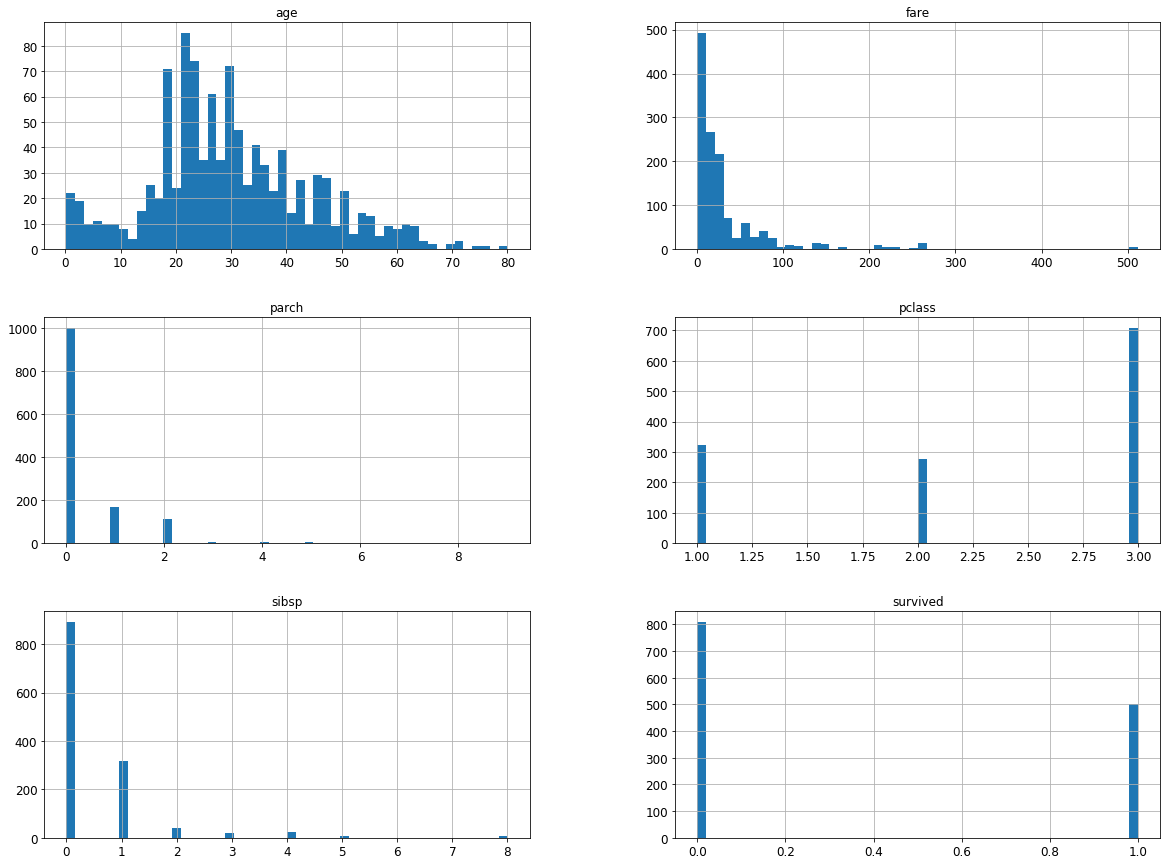

png

创建测试集

切记在看更多详细信息之前，应划分测试集，并把它放到一边，划分数据集有两个方法，一个手动（用 numpy 自己分割），一个自动（sklearn 写好的 api）手动方法适应个性化操作。

数据集过小，单纯的随机创建会产生样本倾斜，采取分层抽样的方式平衡关键属性（看书）

手动划分

import numpy as np

## For illustration only. Sklearn has train_test_split()
def split_train_test(data, test_ratio):
    shuffled_indices = np.random.permutation(len(data))
    test_set_size = int(len(data) * test_ratio)
    test_indices = shuffled_indices[:test_set_size]
    train_indices = shuffled_indices[test_set_size:]
    return data.iloc[train_indices], data.iloc[test_indices]

需要注意的问题：

在每次运行都会生成不同的测试集，解决方法一种是保存下来，另一种是在使用 np.random.permutation() 时先生成随机种子 np.random.seed()
即使确定了随机种子，在数据集更新的时候，依然会出现不同的测试集。解决方法是用对每个实例的标识符哈希化，看书。

##自动划分
from sklearn.model_selection import train_test_split
train_set,test_set = train_test_split(dataset, test_size=0.3, random_state=42)
print(len(train_set),"train +",len(test_set),"test")

916 train + 393 test

详细信息

为了避免发生错误影响数据集，使用训练集的副本。
相关性：主要是看数据趋势是否是正相关和负相关，用散点图很容易就看出来了。其中相关系数可以且只能看出是否是线性相关，散列矩阵则比较强大。对于过多的离散点是否需要采用标准化降低模型拟合时间也有重要指导作用。
属性组合：对于多属性反映同一个事物可以考虑合而为一，或者优化属性。

titanic = train_set.copy()

## 查看数据之间的相关系数
corr_matrix = titanic.corr()
corr_matrix["fare"]

pclass     -0.555562
age         0.137666
sibsp       0.158024
parch       0.214890
fare        1.000000
survived    0.261934
Name: fare, dtype: float64

##数据之间的相关性可视化
from pandas.plotting import scatter_matrix

attributes = ["pclass","age","sibsp","parch","fare","survived"]
scatter_matrix(titanic[attributes], figsize=(24, 16))
plt.show()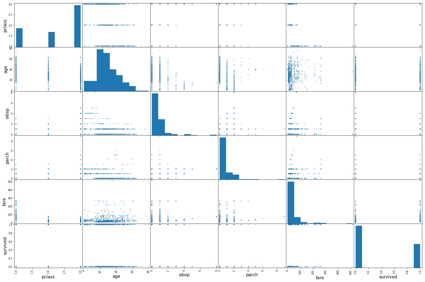

png

##单独拿一个出来看看，为什么感觉青壮年活的多，死的也多，可能是因为基数大吧。
titanic.plot(kind="scatter", x="age", y="survived",
             alpha=0.1)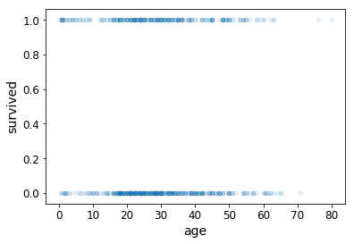

png

数据预处理

预处理的目的：

建立工作流，对于以后更多的数据不必再写代码处理。
逐渐建立自己处理库，复用代码。
易于将数据处理后喂给不同的算法。

在这之前我们需要再一次的将数据与对象（结果）分开

titanic_data = titanic.drop('survived',axis = 1)
titanic_label = titanic['survived'].copy()

数据清洗

缺失值

因为大部分机器学习算法对有缺失值的数据特征不能运作，有下列处理方法：

直接删除整个属性（缺失值过多）.dropna(subset=[‘attribute’])
删除缺失的部分 .drop(‘attribute’, axis = 1)
填充一些值 ,fillna(value)

scikit-learn 提供了 imputer 类进行方便的处理

from sklearn.impute import SimpleImputer
imputer = SimpleImputer(strategy = 'median')
num_attribs = ['pclass', 'age', 'sibsp', 'parch', 'fare']
titanic_num = titanic_data[num_attribs]
imputer.fit(titanic_num)

SimpleImputer(copy=True, fill_value=None, missing_values=nan,
	   strategy='median', verbose=0)

print(imputer.statistics_)
print('*'*30)
print(titanic_data.median())

[  3.   28.    0.    0.   14.5]
******************************
pclass     3.0
age       28.0
sibsp      0.0
parch      0.0
fare      14.5
dtype: float64

X = imputer.transform(titanic_num) #返回结果是numpy，转化为dataframe
titanic_tr = pd.DataFrame(X,columns=titanic_num.columns) #titanic_tr

文本和分类属性

LabelEncoder 直接将不同的标签转化为不同的数字，但是这有一个问题，数字与数字之间是有联系的，而标签与标签之间的联系和数字不一样，这样就造成了样本偏斜
OneHot 编码能够有效避免上述弊端。因此，一般都采用此方法。文本分类 ->标签分类 ->onehot 分类
文本分类可以直接到 Onehot 分类，运用 LabelBinarizer
这里注意类型，原书中不需要转换成 str，这里需要，并且还要转化成 array 用 reshape 方法。

from sklearn.preprocessing import OneHotEncoder
cat_attribs = ["embarked"]
titanic_data.embarked.fillna("Q",inplace = True)
titanic_cat = titanic_data[cat_attribs]
encoder = OneHotEncoder()
titanic_cat_1hot = encoder.fit_transform(np.array(titanic_cat.astype(str)).reshape(-1,1))

encoder.categories_

[array(['C', 'Q', 'S'], dtype=object)]

## 原来返回的是稀疏矩阵，对于大规模的数据存储很有好处。可以用toarray改成下列形式
print(titanic_cat_1hot.toarray())

[[ 0.  0.  1.]
 [ 0.  0.  1.]
 [ 0.  0.  1.]
 ...,
 [ 0.  0.  1.]
 [ 0.  0.  1.]
 [ 0.  0.  1.]]

自定义变换添加额外属性

from sklearn.base import BaseEstimator, TransformerMixin

class CombinedAttributesAdder(BaseEstimator, TransformerMixin):
    def __init__(self, add_bedrooms_per_room = True): # no *args or **kargs
        self.add_bedrooms_per_room = add_bedrooms_per_room
    def fit(self, X, y=None):
        return self  # nothing else to do
    def transform(self, X, y=None):
        rooms_per_household = X[:, rooms_ix] / X[:, household_ix]
        population_per_household = X[:, population_ix] / X[:, household_ix]
        if self.add_bedrooms_per_room:
            bedrooms_per_room = X[:, bedrooms_ix] / X[:, rooms_ix]
            return np.c_[X, rooms_per_household, population_per_household,
                         bedrooms_per_room]
        else:
            return np.c_[X, rooms_per_household, population_per_household]

attr_adder = CombinedAttributesAdder(add_bedrooms_per_room=False)
housing_extra_attribs = attr_adder.transform(housing.values)

管道

from sklearn.pipeline import Pipeline
from sklearn.preprocessing import StandardScaler

num_pipeline = Pipeline([
        ('imputer', SimpleImputer(strategy="median")),
        #('attribs_adder', CombinedAttributesAdder()),
        ('std_scaler', StandardScaler()),
    ])
titanic_num_tr = num_pipeline.fit_transform(titanic_num)

titanic_num_tr

array([[ 0.82524778, -0.07091793, -0.49861561, -0.43255344, -0.47409151],
	   [ 0.82524778, -0.23259583, -0.49861561, -0.43255344, -0.48861599],
	   [-0.36331663, -0.79846845, -0.49861561, -0.43255344, -0.14564735],
	   ...,
	   [ 0.82524778, -0.03049846, -0.49861561, -0.43255344, -0.33319441],
	   [ 0.82524778, -0.23259583, -0.49861561, -0.43255344, -0.48806282],
	   [ 0.82524778, -0.07091793, -0.49861561, -0.43255344, -0.48861599]])

from sklearn.compose import ColumnTransformer

full_pipeline = ColumnTransformer([
        ("num", num_pipeline, num_attribs),
        ("cat", OneHotEncoder(), cat_attribs),
    ])
titanic_prepared = full_pipeline.fit_transform(titanic_data)

titanic_prepared.shape #(916,8)

选择和训练模型

这里选用的是线性回归模型，仅仅是试一试，可以看出效果是相当不好.显然，一个分类问题用回归模型来训练，显然是错误的
线性回归模型常用均方根来表示误差
随机梯度下降分类器模型看得出有点效果，性能通常用召回率，准确率来表征，这里没有过多展示。

from sklearn.linear_model import LinearRegression
lin_reg = LinearRegression()
lin_reg.fit(titanic_prepared, titanic_label)

LinearRegression(copy_X=True, fit_intercept=True, n_jobs=None,
		 normalize=False)

some_data = test_set.iloc[:5]
some_labels = titanic_label.iloc[:5]
some_data_prepared = full_pipeline.transform(some_data)
print("Predictions:", lin_reg.predict(some_data_prepared))

print("Labels:", list(some_labels))

Labels: [0, 0, 1, 0, 0]

from sklearn.metrics import mean_squared_error

titanic_predictions = lin_reg.predict(titanic_prepared)
lin_mse = mean_squared_error(titanic_label, titanic_predictions)
lin_rmse = np.sqrt(lin_mse)
lin_rmse # 0.44458368170220458

from sklearn.metrics import mean_absolute_error

lin_mae = mean_absolute_error(titanic_label, titanic_predictions)
lin_mae #    0.39530930007177417

from sklearn.tree import DecisionTreeRegressor

tree_reg = DecisionTreeRegressor(random_state=42)
tree_reg.fit(titanic_prepared, titanic_label)
housing_predictions = tree_reg.predict(titanic_prepared)
tree_mse = mean_squared_error(titanic_label, titanic_predictions)
tree_rmse = np.sqrt(tree_mse)
tree_rmse #    0.44458368170220458

from sklearn.linear_model import SGDClassifier

sgd_clf = SGDClassifier(max_iter=5, random_state=42)
sgd_clf.fit(titanic_prepared, titanic_label)

SGDClassifier(alpha=0.0001, average=False, class_weight=None,
	   early_stopping=False, epsilon=0.1, eta0=0.0, fit_intercept=True,
	   l1_ratio=0.15, learning_rate='optimal', loss='hinge', max_iter=5,
	   n_iter=None, n_iter_no_change=5, n_jobs=None, penalty='l2',
	   power_t=0.5, random_state=42, shuffle=True, tol=None,
	   validation_fraction=0.1, verbose=0, warm_start=False)

print("Predictions:", sgd_clf.predict(some_data_prepared)) #    Predictions: [0 0 0 0 1]

print("Labels:", list(some_labels)) #    Labels: [0, 0, 1, 0, 0]

优化模型

用的最多的就是交叉验证
其次是对模型调参，参数的搜索
最后是对各个模型融合进行预测,得到一个最好的模型就完事了

交叉验证

from sklearn.model_selection import cross_val_score

scores = cross_val_score(tree_reg, titanic_prepared, titanic_label,
                         scoring="neg_mean_squared_error", cv=5)
tree_rmse_scores = np.sqrt(-scores)

def display_scores(scores):
    print("Scores:", scores)
    print("Mean:", scores.mean())
    print("Standard deviation:", scores.std())

display_scores(tree_rmse_scores) #    array([ 0.62210924,  0.59404   ,  0.63470788,  0.58847198,  0.56893364])

参数搜索

给参数自动进行比较，选出最优参数
随机搜索最优参数

模型建立

from sklearn.ensemble import RandomForestRegressor

forest_reg = RandomForestRegressor(random_state=42)
forest_reg.fit(titanic_prepared, titanic_label)

RandomForestRegressor(bootstrap=True, criterion='mse', max_depth=None,
		   max_features='auto', max_leaf_nodes=None,
		   min_impurity_decrease=0.0, min_impurity_split=None,
		   min_samples_leaf=1, min_samples_split=2,
		   min_weight_fraction_leaf=0.0, n_estimators=10, n_jobs=None,
		   oob_score=False, random_state=42, verbose=0, warm_start=False)

titanic_predictions = forest_reg.predict(titanic_prepared)
forest_mse = mean_squared_error(titanic_label, titanic_predictions)
forest_rmse = np.sqrt(forest_mse)
forest_rmse #    0.24601252278498684

给定参数搜索

from sklearn.model_selection import GridSearchCV

param_grid = [
    # try 12 (3×4) combinations of hyperparameters
    {'n_estimators': [3, 10, 30], 'max_features': [2, 4, 6, 8]},
    # then try 6 (2×3) combinations with bootstrap set as False
    {'bootstrap': [False], 'n_estimators': [3, 10], 'max_features': [2, 3, 4]},
  ]

forest_reg = RandomForestRegressor(random_state=42)
## train across 5 folds, that's a total of (12+6)*5=90 rounds of training
grid_search = GridSearchCV(forest_reg, param_grid, cv=5,
                           scoring='neg_mean_squared_error', return_train_score=True)
grid_search.fit(titanic_prepared,titanic_label)

GridSearchCV(cv=5, error_score='raise-deprecating',
	   estimator=RandomForestRegressor(bootstrap=True, criterion='mse', max_depth=None,
		   max_features='auto', max_leaf_nodes=None,
		   min_impurity_decrease=0.0, min_impurity_split=None,
		   min_samples_leaf=1, min_samples_split=2,
		   min_weight_fraction_leaf=0.0, n_estimators='warn', n_jobs=None,
		   oob_score=False, random_state=42, verbose=0, warm_start=False),
	   fit_params=None, iid='warn', n_jobs=None,
	   param_grid=[{'n_estimators': [3, 10, 30], 'max_features': [2, 4, 6, 8]}, {'bootstrap': [False], 'n_estimators': [3, 10], 'max_features': [2, 3, 4]}],
	   pre_dispatch='2*n_jobs', refit=True, return_train_score=True,
	   scoring='neg_mean_squared_error', verbose=0)

grid_search.best_params_ #    {'max_features': 8, 'n_estimators': 30}

grid_search.best_estimator_

RandomForestRegressor(bootstrap=True, criterion='mse', max_depth=None,
		   max_features=8, max_leaf_nodes=None, min_impurity_decrease=0.0,
		   min_impurity_split=None, min_samples_leaf=1,
		   min_samples_split=2, min_weight_fraction_leaf=0.0,
		   n_estimators=30, n_jobs=None, oob_score=False, random_state=42,
		   verbose=0, warm_start=False)

cvres = grid_search.cv_results_
for mean_score, params in zip(cvres["mean_test_score"], cvres["params"]):
    print(np.sqrt(-mean_score), params)

0.497131363834 {'max_features': 2, 'n_estimators': 3}
0.480945066964 {'max_features': 2, 'n_estimators': 10}
0.467748997902 {'max_features': 2, 'n_estimators': 30}
0.502741663175 {'max_features': 4, 'n_estimators': 3}
0.476083472783 {'max_features': 4, 'n_estimators': 10}
0.464671414883 {'max_features': 4, 'n_estimators': 30}
0.500998128825 {'max_features': 6, 'n_estimators': 3}
0.4723270942 {'max_features': 6, 'n_estimators': 10}
0.464692668366 {'max_features': 6, 'n_estimators': 30}
0.491656899488 {'max_features': 8, 'n_estimators': 3}
0.468153614704 {'max_features': 8, 'n_estimators': 10}
0.462619186958 {'max_features': 8, 'n_estimators': 30}
0.534684910518 {'bootstrap': False, 'max_features': 2, 'n_estimators': 3}
0.516588728861 {'bootstrap': False, 'max_features': 2, 'n_estimators': 10}
0.535750828291 {'bootstrap': False, 'max_features': 3, 'n_estimators': 3}
0.516586118116 {'bootstrap': False, 'max_features': 3, 'n_estimators': 10}
0.535870542379 {'bootstrap': False, 'max_features': 4, 'n_estimators': 3}
0.512291127875 {'bootstrap': False, 'max_features': 4, 'n_estimators': 10}

随机参数搜索

from sklearn.model_selection import RandomizedSearchCV
from scipy.stats import randint

param_distribs = {
        'n_estimators': randint(low=1, high=200),
        'max_features': randint(low=1, high=8),
    }

forest_reg = RandomForestRegressor(random_state=42)
rnd_search = RandomizedSearchCV(forest_reg, param_distributions=param_distribs,
                                n_iter=10, cv=5, scoring='neg_mean_squared_error', random_state=42)
rnd_search.fit(titanic_prepared,titanic_label)

RandomizedSearchCV(cv=5, error_score='raise-deprecating',
		  estimator=RandomForestRegressor(bootstrap=True, criterion='mse', max_depth=None,
		   max_features='auto', max_leaf_nodes=None,
		   min_impurity_decrease=0.0, min_impurity_split=None,
		   min_samples_leaf=1, min_samples_split=2,
		   min_weight_fraction_leaf=0.0, n_estimators='warn', n_jobs=None,
		   oob_score=False, random_state=42, verbose=0, warm_start=False),
		  fit_params=None, iid='warn', n_iter=10, n_jobs=None,
		  param_distributions={'n_estimators': <scipy.stats._distn_infrastructure.rv_frozen object at 0x000001D1B51B6198>, 'max_features': <scipy.stats._distn_infrastructure.rv_frozen object at 0x000001D1B51B6978>},
		  pre_dispatch='2*n_jobs', random_state=42, refit=True,
		  return_train_score='warn', scoring='neg_mean_squared_error',
		  verbose=0)

cvres = rnd_search.cv_results_
for mean_score, params in zip(cvres["mean_test_score"], cvres["params"]):
    print(np.sqrt(-mean_score), params)

0.464039645236 {'max_features': 7, 'n_estimators': 180}
0.471855747311 {'max_features': 5, 'n_estimators': 15}
0.469662076234 {'max_features': 3, 'n_estimators': 72}
0.4681528737 {'max_features': 5, 'n_estimators': 21}
0.464796324533 {'max_features': 7, 'n_estimators': 122}
0.469440835097 {'max_features': 3, 'n_estimators': 75}
0.469061926876 {'max_features': 3, 'n_estimators': 88}
0.464095537716 {'max_features': 5, 'n_estimators': 100}
0.465712273605 {'max_features': 3, 'n_estimators': 150}
0.521753546174 {'max_features': 5, 'n_estimators': 2}

feature_importances = grid_search.best_estimator_.feature_importances_
feature_importances

array([ 0.08056266,  0.35015732,  0.0670613 ,  0.052615  ,  0.39991869,
		0.01900031,  0.00781355,  0.02287116])

其他

pipeline 可以把训练模型这个过程也加进去
可以用 sklearn 的模块保存模型，加载模型

full_pipeline_with_predictor = Pipeline([
        ("preparation", full_pipeline),
        ("linear", LinearRegression())
    ])

full_pipeline_with_predictor.fit(titanic_data,titanic_label)
full_pipeline_with_predictor.predict(some_data) #    array([ 0.14901183,  0.37719866,  0.18577842,  0.18589226,  0.29765968])

my_model = full_pipeline_with_predictor

from sklearn.externals import joblib
joblib.dump(my_model, "my_model.pkl") # DIFF
##...
my_model_loaded = joblib.load("my_model.pkl") # DIFF